Absolute Solvation Protocol

Overview

The AbsoluteSolvationProtocol calculates the free energy change associate with transferring a molecule from vacuum into a solvent.

Note

Currently, water is the only supported solvent, however, more solvents might be possible in the future.

The absolute solvation free energy is calculated through a thermodynamic cycle. In this cycle, the interactions of the molecule are decoupled, meaning turned off, using a partial annihilation scheme (see below) both in the solvent and in the vacuum phases. The absolute solvation free energy is then obtained via summation of free energy differences along the thermodynamic cycle.

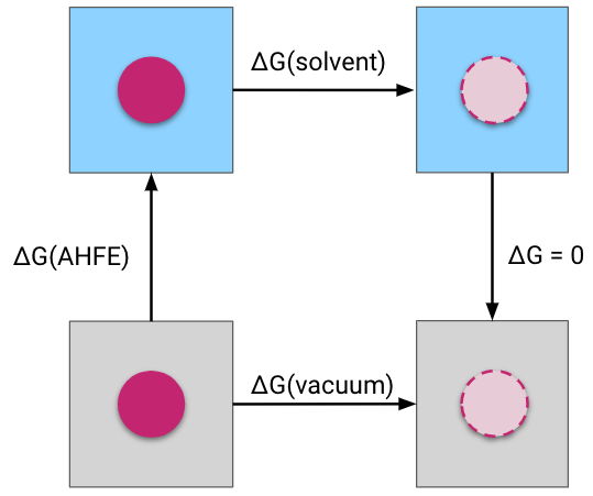
Thermodynamic cycle for the absolute solvation free energy protocol.

Scientific Details

Partial annihilation scheme

In the AbsoluteSolvationProtocol the coulombic interactions of the molecule are fully turned off (annihilated). The Lennard-Jones interactions are instead decoupled, meaning the intermolecular interactions turned off, keeping the intramolecular Lennard-Jones interactions.

The lambda schedule

Molecular interactions are turned off during an alchemical path using a discrete set of lambda windows. The electrostatic interactions are turned off first, followed by the decoupling of the Lennard-Jones interactions.

A soft-core potential is applied to the Lennard-Jones potential to avoid instablilites in intermediate lambda windows. Both the soft-core potential functions from Beutler et al. [1] and from Gapsys et al. [2] are available and can be specified in the alchemical_settings.softcore_LJ settings (default: gapsys).

Lambda schedules for the solvent and vacuum legs are defined by the lambda_elec and lambda_vdw entries of solvent_lambda_settings and vacuum_lambda_settings respectively. A value of 0.0 means the interactions are fully on, and 1.0 means they are fully decoupled (or annihilated).

Note

The lambda settings have a lambda_restraints entry that is ignored for the AbsoluteSolvationProtocol.

By default, the solvent leg uses 14 lambda windows, while the vacuum leg uses only 5 lambda windows. This is because there are no intermolecular interactions to scale in vacuum. This means that only the electrostatic interactions, which are annihilated, need to be turned off gradually. Since decoupling the Lennard-Jones interactions has no effect in vacuum, lambda_vdw is simply switched to 1.0 in the final window of the vacuum schedule.

Note

If alchemical_settings.annihilate_sterics is set to True, the intramolecular Lennard-Jones interactions are also turned off. In this case the default vacuum lambda schedule is not appropriate, and intermediate lambda_vdw windows should be added to vacuum_lambda_settings.

The number of lambda windows in each leg must match the number of replicas set in solvent_simulation_settings.n_replicas and vacuum_simulation_settings.n_replicas.

Simulation overview

The ProtocolDAG of the AbsoluteSolvationProtocol contains ProtocolUnits from both the vacuum and solvent transformations. This means that both legs of the thermodynamic cycle are constructed and run concurrently in the same ProtocolDAG. This is different from the RelativeHybridTopologyProtocol where the ProtocolDAG only runs a single leg of a thermodynamic cycle. If multiple protocol_repeats are run (default: protocol_repeats=3), the ProtocolDAG contains multiple ProtocolUnits of both vacuum and solvent transformations.

Simulation steps

Each ProtocolUnit (whether vacuum or solvent) carries out the following steps:

1. Parameterize the system using OpenMMForceFields and Open Force Field.

2. Equilibrate the fully interacting system using a short MD simulation using the same approach as the PlainMDProtocol (in the solvent leg this will include rounds of NVT and NPT equilibration).

3. Create an alchemical system.

4. Minimize the alchemical system.

5. Equilibrate and production simulate the alchemical system using the chosen multistate sampling method (under NPT conditions if solvent is present).

6. Analyze results for the transformation.

Note: three different types of multistate sampling (i.e. replica swapping between lambda states) methods can be chosen; HREX, SAMS, and independent (no lambda swaps attempted). By default the HREX approach is selected, this can be altered using solvent_simulation_settings.sampler_method or vacuum_simulation_settings.sampler_method (default: repex).

Simulation details

Here are some details of how the simulation is carried out which are not detailed in the AbsoluteSolvationSettings:

• The protocol applies a LangevinMiddleIntegrator which uses Langevin dynamics, with the LFMiddle discretization [3].

• A MonteCarloBarostat is used in the NPT ensemble to maintain constant pressure.

Getting the free energy estimate

The free energy differences are obtained from simulation data using the MBAR estimator (multistate Bennett acceptance ratio estimator) as implemented in the PyMBAR package. Both the MBAR estimates of the two legs of the thermodynamic cycle, and the overall absolute solvation free energy (of the entire cycle) are obtained, which is different compared to the results in the RelativeHybridTopologyProtocol where results from two legs of the thermodynamic cycle are obtained separately.

In addition to the estimates of the free energy changes and their uncertainty, the protocol also returns some metrics to help assess convergence of the results, these are detailed in the multistate analysis section.

Analysis

As with the RelativeHybridTopologyProtocol, the protocol performs both energetic and structural analysis automatically after each simulation repeat. The energetic analysis (MBAR overlap matrix, replica exchange statistics, forward/reverse convergence) is identical to that described in the multistate analysis section.

Structural analysis

After each simulation, the protocol automatically analyzes the production trajectories.

Note

No structural analysis is currently carried out for the vacuum leg. This will be fixed in a future version of openfe.

For each lambda state, the Ligand RMSD is computed: a symmetry-corrected RMSD of the ligand relative to the first production frame. A symmetry-corrected RMSD is used to account for equivalent atom orderings in symmetric molecules (e.g. a flipping phenyl ring) instead of a standard mass-weighted RMSD.

Results are saved as an NPZ file (structural_analysis.npz) and a plot (ligand_RMSD.png) is generated automatically. To customize the analysis, the frame stride can be configured via analysis_settings.skip in AbsoluteSolvationSettings.

Note

This analysis requires the ligand atoms to be included in the trajectory output (controlled by output_indices in solvent_output_settings). If no ligand atoms are written to the trajectory, the analysis is skipped and a structural_analysis_error entry is added to the results instead.

For further guidance on interpreting this plot, see the multistate analysis section of the hybrid topology protocol documentation.

See Also

Setting up AFE calculations

• Defining the Protocol

Tutorials

• Absolute Hydration Free Energies tutorial

Cookbooks

Cookbooks

API Documentation

• OpenMM Absolute Solvation Free Energy

• OpenMM Protocol Settings

References

• pymbar

• yank

• OpenMMTools

• OpenMM

[1]

Avoiding singularities and numerical instabilities in free energy calculations based on molecular simulations, T.C. Beutler, A.E. Mark, R.C. van Schaik, P.R. Greber, and W.F. van Gunsteren, Chem. Phys. Lett., 222 529–539 (1994)

[2]

New Soft-Core Potential Function for Molecular Dynamics Based Alchemical Free Energy Calculations, V. Gapsys, D. Seeliger, and B.L. de Groot, J. Chem. Theor. Comput., 8 2373-2382 (2012)

[3]

Unified Efficient Thermostat Scheme for the Canonical Ensemble with Holonomic or Isokinetic Constraints via Molecular Dynamics, Zhijun Zhang, Xinzijian Liu, Kangyu Yan, Mark E. Tuckerman, and Jian Liu, J. Phys. Chem. A 2019, 123, 28, 6056-6079